ML: Building a simple classifier (Titanic pt.1)
Learning Machine Learning is an intimidating task - there is simply way too much to learn, too many tools, technologies and techniques to grasp. On the other hand, pioneers of the discipline are continuously releasing more and more tools that help with that. Python ecosystem is a great example - in this article we will attempt to solve the Kaggle Titanic challenge using as little code and knowledge as possible.
This article is part of Titanic series - a short series on basic ML concepts based on the famous Titanic Kaggle challenge
the problem
This exercise is about predicting whether people would survive the unfortunate Titanic disaster.
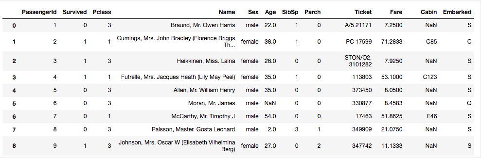
Train data example:
the solution
We will jump straight in - I will not do any real data exploration here, we can save that for later - just from opening the input file we can easily pick up the obvious columns that can be (almost) directly used for simple predictions whether a person would survive the disaster or not.
Let’s begin with the simplest - importing the data.
1 2 3 | import pandas as pd train = pd.read_csv("train.csv") test = pd.read_csv("test.csv") |
We need to choose the columns we wish to use for creating the prediction model - i.e. the columns used for predictions. Let’s use the most obvious four - Fare, Sex, Age and Pclass (ticket class) and prepare data frames of features and results.
1 2 3 | columns = ["Fare", "Sex", "Pclass", "Age"] X_all = train[columns] y_all = train["Survived"] |
Brief look at the data shows us that before we continue, we have to change the string Sex column into a numeric format - so that the ML math magic can happen. To do that, we can simply use the pd.factorize method from pandas like so:
1 2 | train["Sex"] = pd.factorize(train["Sex"])[0] test["Sex"] = pd.factorize(test["Sex"])[0] |
Another detail we have to handle before moving on is missing values in the Fare and Age columns. For simplicity sake we can fill in the missing values with the average value of the column.
1 2 3 4 | train["Fare"] = train["Fare"].fillna((train["Fare"].mean())) test["Fare"] = test["Fare"].fillna((test["Fare"].mean())) train["Age"] = train["Age"].fillna((train["Age"].mean())) test["Age"] = test["Age"].fillna((test["Age"].mean())) |
Now the data is ready, we can proceed and prepare our training and test sets. The most common and simple way of doing so is to use the training set which contains the results and splitting it into a train and test part (we will call them X_train and X_test for features sets, and y_train and y_test for the answers). Then we can use these for validating our model, and after we are happy with out model we train on the complete train set and predict on the test set which is missing the “right answers”.
Here we split the train set 80/20.
1 2 | from sklearn.model_selection import train_test_split X_train, X_test, y_train, y_test = train_test_split(X_all, y_all, test_size = 0.2, random_state = 0) |
Now we can proceed with creating the classifier, fitting the data and making our first predictions. We are using one of the basic ML Logistic Regression algorithms.
1 2 3 4 | from sklearn.linear_model import LogisticRegression classifier = LogisticRegression(random_state = 0, solver="lbfgs", max_iter = 100) classifier.fit(X_train, y_train) prediction = prediction = classifier.predict(X_test) |
Voila! Our first logistic regression classifier is predicting something! But what is it predicting and how good are the predictions? We can use a simple Confusion Matrix tool and calculate the accuracy of our predictions based on true positives and true negatives.
1 2 3 4 | from sklearn.metrics import confusion_matrix cm = confusion_matrix(y_test, prediction) print(f"Confusion matrix:\n{cm}") print(f"Accuracy: {(cm[1][1] + cm[0][0]) / len(y_test)}") |
1 2 3 4 5 | python simplest.py Confusion matrix: [[94 16] [18 51]] Accuracy: 0.8100558659217877 |
We are getting accuracy on our validation train set of over 81%! Not bad for such a simple model!
Let’s continue and fit on our whole train set and predict the unknown test values.
1 2 | classifier.fit(X_all, y_all) prediction = classifier.predict(test[columns]) |
Now that the test prediction is done we can prepare the submission data.
1 2 3 | submission_df = {"PassengerId": test["PassengerId"], "Survived": prediction} submission = pd.DataFrame(submission_df) submission.to_csv(f"predictions/titanic_simplest.csv", index=False) |
Submitting the generated file to Kaggle scores us a decent 75.1%.
Code for this simplest model can be found here -it’s 40 lines of code only, including the comments!.
improvements
There are many things one could try to improve on the performance of the classifier, we will look into some of these in next articles:
- Use One Hot Encoding - a standard approach for categorical data and apply it to categorical columns like Sex or Embarked.
- Feature engineering - extracting and/or combining data from columns to come up with new features that might describe the reality better than the raw data. Example - extract deck information from cabin number, include caluclated family size feature, extract and categorize title, categorize age.
- Try using different models - different models can produce different results as they are optimized for different scenarios. Choosing the right algorithm can do wonders.
This article is part of Titanic series - a short series on basic ML concepts based on the famous Titanic Kaggle challenge